Variable Selection (Part 1)

<-PREVIOUS PAGE NEXT PAGE ->

In the world there is noise. Too many unnecessary variables can distract our model and take away from desired performance. One of the most important aspects of any machine learning project, especially when using data from the real world, is learning dimensionality reduction, or how to meaningfully reduce the our set of variables to its most valuable components.

Dimensionality reduction, understanding the base variables and how they work together, can prove to be a major source of help on this journey to find the principal set of variables.

It is most important to first establish how each of our variables are correlated with one another. Does batting average correspond with the weather? Does strikeout percentage correspond with a lower earned run average? Finding correlations of the variables and seeing the behavior of all the original variables can help us give us good insight to which variables are of interest in this case.

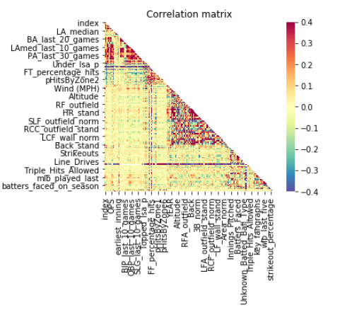
The correlation map below gathers all the Pearson correlations of our variables using the merged data gathered from our hitting, weather, stadium, and pitching datasets. Let’s take a look at how our hundreds (approximately 200 of them) of variables and see how they relate:

As expected, there is a lot of noise and nonsense! How do we make sense of too much information? There does seem to be significant clusters of correlatory variables that are worth looking at. Overall, however, with over 200 different variables, a display in one map can be extremely difficult to interpret. Thus, we will have to cut down more variables to see a good trace of variable behavior.

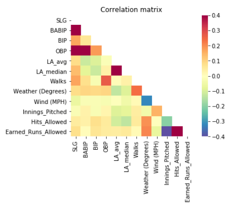
Let’s take a step back, and intuitively figure out what would make a desirable varaible set. We can throw fancy dimensionality reduction techniques at our variable set, but in many cases, gathering the intuitive variables from the most basic level can be a great first step to achieving a succesful model. Batting average, contact percentage, batting average per ball put into play, weather, average launch angle, strikeout percentage, hits allowed on average, and innings pitched on average seems like a great place to start. For better understanding, here is a list of all the variables included:

‘SLG’,‘BABIP’,‘BIP’,‘OBP’,‘LA_avg’,‘LA_median’,‘Walks’,‘Venue’,‘Weather (Degrees)’,‘Wind (MPH)’,‘Innings_Pitched’,‘Hits_Allowed’, ‘Earned_Runs_Allowed’

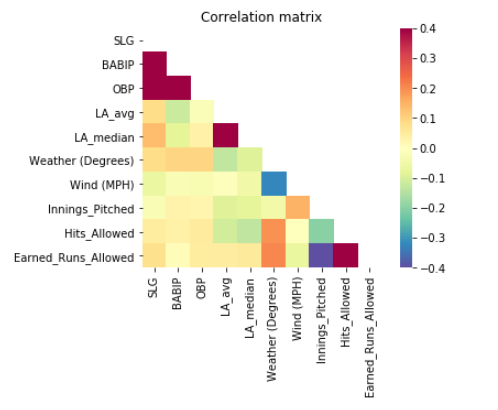
In this correlation map, there are some interesting relationships with some variables but not all. For example, it doesn’t seem like Walks have a significant effect with everything else, and neither does Ball in play percentage. Let’s remove those variables.

In this correlation map we see a good trace of the behavior variables of interest given their relationships with the other variables. This is a great starting point for our model. We can now move forward with adding and taking away more variables and seeing how our model performs in response!

In conclusion, these selected variables prove to be worthy for our model. At least at this point…

<-PREVIOUS PAGE NEXT PAGE ->